Schur's lemma in piecewise linear
Hoover your cursor over the pictures below to get started! Explanations for what is going on can be found at the end of the page: jump to backgroundPut your cursor over a diagram, then the program will take that vector in \(L_{i}\), include it into \(R\), run ReLU or any of the other maps, then project back down to all of the simples. The trivial and sign representations are included along the real axis (any imaginary component of the cursor is ignored). The scaling checkbox attempts to scale the outputs so that the length of the image of one is equal to one in each simple. This is recommended as the coefficients of the projectors scale the maps quite drastically. For example, parametric ReLU is almost linear and one cannot tell the difference to \(f\colon x\mapsto x\) in an unscaled plot.
Interaction graphs
Use your cursor to change the size and some other features of the graphs graphs. (These are computed live and might need some time to load.)\(L_{1}\) to trivial and sign as a map
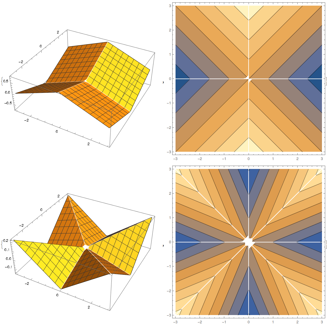
Use your cursor to change the some features of the maps below. (These are computed live and might need some time to load.)For the sign \(C_{n}\)-representation the picture is a “monkey saddle”; here \(n=4\) and \(n=8\):
To get the notebook for the sign representation click here.
Background
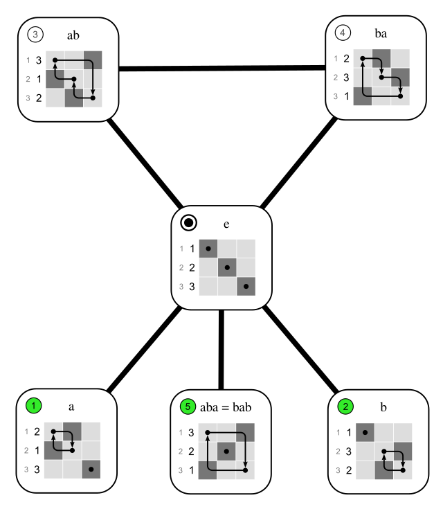
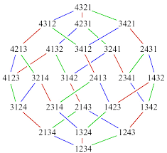
This page is about the cyclic group. For the dihedral group or the symmetric group click on the associated picture below.
Everything is based on fabulous work of Joel Gibson related to Joel's
Lievis. See also some slides.
For a nice illustration, and much more, why linear maps do not go very well with neural networks see here.
Here is a bit of mathematical background on what is going on.
- Our ground field is \(\mathbb{R}\). Fix \(n\in\mathbb{Z}_{\geq 1}\), and depending on parity, let \(m\) be defined by \(n=2m\) or \(n=2m+1\). Let \(\theta=2\pi/n\); rotation is always clockwise.
- Let \(C_{n}=\mathbb{Z}/n\mathbb{Z}=\langle a|a^{n}=1\rangle\) be the cyclic group of order \(n\).
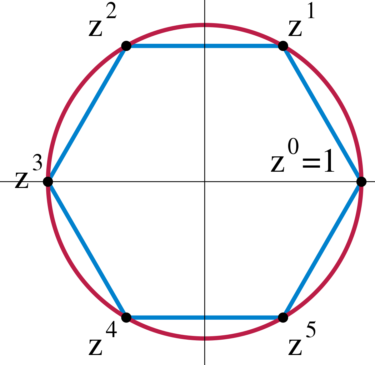
- This group acts on the \(n\) dimensional \(\mathbb{R}\)-vector space \(R=\mathbb{R}\{x_{0},\dots,x_{n-1}\}\) by cyclic permutation of the coordinates: \(a\centerdot x_{i}=x_{i+1}\), reading indexes modulo \(n\). This \(C_{n}\)-representation is called the regular representation.
- For \(n\) even there are precicely \(m\) nonequivalent simple real \(C_{n}\)-representations: \[L_{0}\leftrightsquigarrow\text{trivial},L_{1}\leftrightsquigarrow\text{rotation by }\theta,\dots,L_{m-1}\leftrightsquigarrow\text{rotation by }(m-1)\theta, L_{m}\leftrightsquigarrow\text{sign}\] These are of dimensions \(1,2,\dots,2,1\).
- For \(n\) odd the same is true, but \(L_{m}\) is not the sign \(C_{n}\)-representation (there is no such representation) but rather another two dimensional \(C_{n}\)-representation. The dimension sequence is \(1,2,\dots,2\).
- The Artin–Wedderburn decomposition of \(R\) into simple real \(C_{n}\)-representation is as follows: \[R\cong \underbrace{L_{0}}_{1d}\oplus \underbrace{L_{1}\oplus\dots\oplus L_{m-1}}_{2d}\oplus \underbrace{L_{m}}_{1d}\] for \(n\) even, and \[R\cong \underbrace{L_{0}}_{1d}\oplus \underbrace{L_{1}\oplus\dots\oplus L_{m}}_{2d}\] for \(n\) odd.
- The base change matrices realizing these Artin–Wedderburn decompositions are easy to get from the character table of \(C_{n}\). Here is one such matrix, the inclusion matrix, for \(n=5\): \[ include \leftrightsquigarrow \begin{pmatrix} 1 & -\sin(2\pi 1/5) & \cos(2\pi 1/5) & -\sin(4\pi 1/5) & \cos(4\pi 1/5) \\ 1 & -\sin(2\pi 2/5) & \cos(2\pi 2/5) & -\sin(4\pi 1/5) & \cos(4\pi 2/5) \\ 1 & -\sin(2\pi 3/5) & \cos(2\pi 3/5) & -\sin(4\pi 1/5) & \cos(4\pi 3/5) \\ 1 & -\sin(2\pi 4/5) & \cos(2\pi 4/5) & -\sin(4\pi 1/5) & \cos(4\pi 4/5) \\ 1 & -\sin(2\pi 5/5) & \cos(2\pi 5/5) & -\sin(4\pi 1/5) & \cos(4\pi 5/5) \end{pmatrix}. \] The general pattern is similar.
In the demonstration above shows what happens to certain piecewise linear maps upon decomposition, that is, the above calculates the map
\[L_{i}\xrightarrow{include}R\xrightarrow{\hspace{0.5cm}f\hspace{0.5cm}}R\xrightarrow{project}L_{j}\]
for the maps \(f\colon x\mapsto x\) (this is a linear map), \(ReLU\colon x\mapsto\max(x,0)\)
(this map is called ReLU)
and \(Abs\colon x\mapsto\max(x,-x)\) (this map is called
absolute value), and \(\text{leaky} ReLU\colon x\mapsto\max(x,0.01x)\) as well as \(\text{parametric} ReLU\colon x\mapsto\max(x,0.99x)\)
(these maps are special cases of the map called parametric ReLU, see also
leaky ReLU).
Using the above basis, these maps are extended
componentwise to \(R\), and the resulting maps are \(C_{n}\)-equivariant. Any two of these form a basis over \(\mathbb{R}\) of the space of all piecewise linear maps
\(\mathbb{R}\to\mathbb{R}\). The order above means the order of the action matrix of the generator \(a\).
For historical reasons (and because its fun) we added Tanh as well, although this map is not piecewise linear
The interaction graph (on \(R\)) of a \(C_{n}\)-equivariant map \(f\) is the graph with vertices indexed by the simple real constituents \(L_{i}\) of \(R\), counted with multiplicities, and an edge from \(L_{i}\) to \(L_{j}\) if the map \[L_{i}\xrightarrow{include}R\xrightarrow{\hspace{0.5cm}f\hspace{0.5cm}}R\xrightarrow{project}L_{j}\] is not zero.
The interaction graph for \(f\colon x\mapsto x\), or any other \(C_{n}\)-equivariant linear map, is trivial (i.e. we only have isolated vertices with loops), while the intersection graph for PReLU is the same as for ReLU itself. Above are the first few interaction graphs for ReLU (first) and the absolute value (second), where the vertices are labeled \(i\) instead of \(L_{i}\).
The theorem for ReLU is as follows. Define the adjusted order as the one above divided by two if the order itself is even. Call this \(ord^{\prime}\). Then every vertex in the intersection graph has a loop and there is a non-loop edge from \(L_{i}\) to \(L_{j}\) if and only if \(ord(L_{j})\) divides \(ord^{\prime}(L_{i})\) (note that the order and the adjusted order appear here). For the absolute value the theorem reads the same but dropping the forced existence of loops (the order condition itself might give loops as well).
The mapsLet \(n\in\{1,\dots,8\}\). The maps illustrate \[ L_{1}\xrightarrow{include}R\xrightarrow{\hspace{0.5cm}f\hspace{0.5cm}}R\xrightarrow{project}trivial \quad\text{and}\quad L_{1}\xrightarrow{include}R\xrightarrow{\hspace{0.5cm}f\hspace{0.5cm}}R\xrightarrow{project}sign, \] the latter only for \(n\equiv 0\bmod 4\) (the cases \(n\equiv 2\bmod 4\) are similar but skipped). Note that \(\dim_{\mathbb{R}}L_{1}=2\) and the trivial and sign \(C_{n}\)-representations are one dimensional. Thus, we can illustrate the above maps as maps \(\mathbb{R}^{2}\to\mathbb{R}\), which is what is done in the illustrations above. The first plot is a standard 3d plot, the second a contour plot using level sets.
Closing remarks
Finite abelian groupsAbove we discussed the case of cyclic groups, and the discussion below then implies that we understand the case of general finite abelian groups as well. To elaborate, recall that all finite abelian groups are of the form \[ C_{n_{1}}\times\dots\times C_{n_{k}} \cong \mathbb{Z}/n_{1}\mathbb{Z}\times\dots\times\mathbb{Z}/n_{k}\mathbb{Z}, \quad n_{i}\in\mathbb{Z}_{\geq 2}. \] It turns out that products of groups are easy with respect to the above, so the cyclic group case settles the general finite abelian groups as well.
For example, the interaction graph are just product graphs. Explicitly:
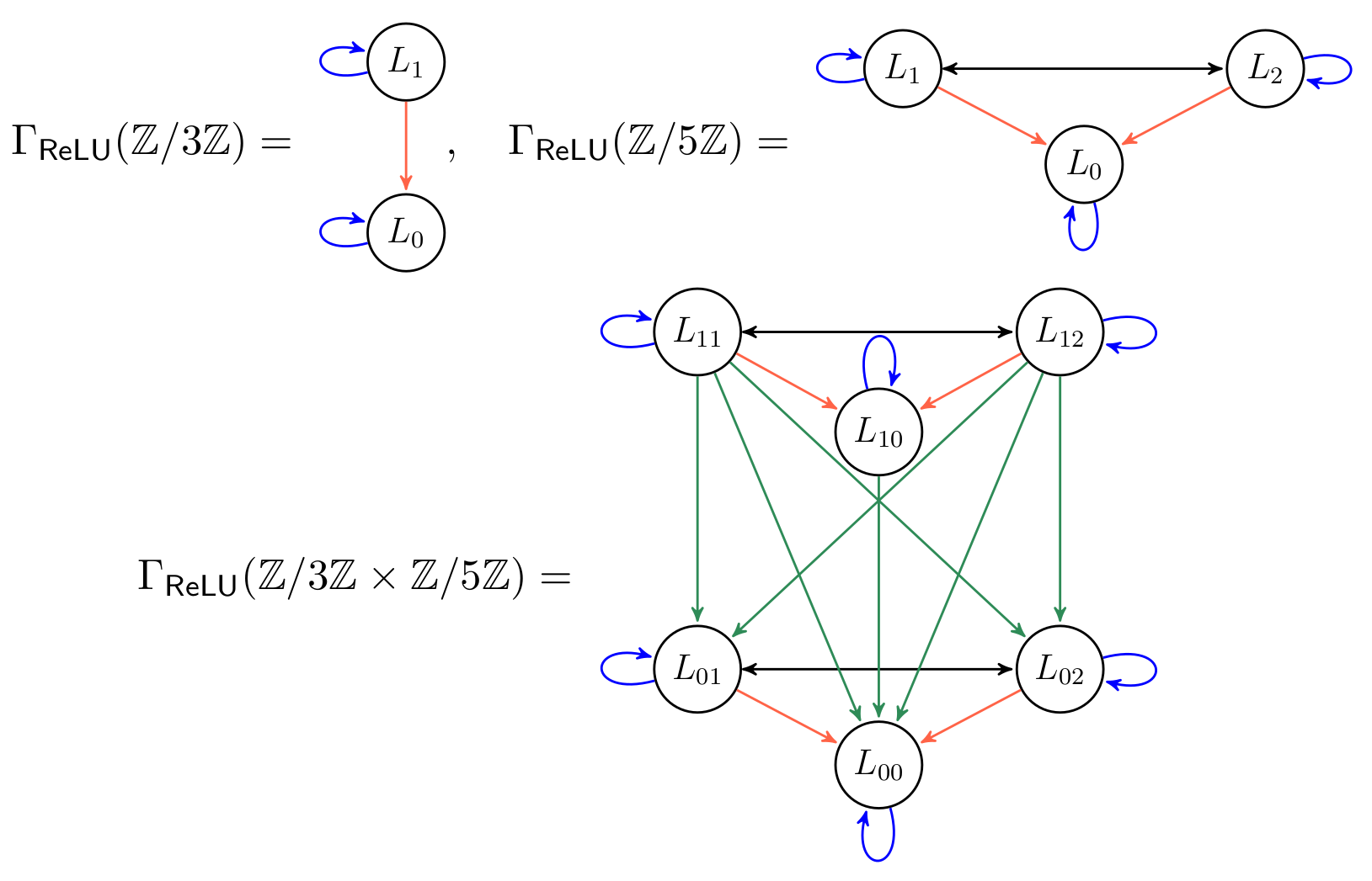
For potential “real-world” applications click here.